Outperform cuBLAS with OpenGL
Writing BLAS routines in fragment shaders.
Table of Contents
Compute libraries, like CUDA and OpenCL, are responsible for handling the compute pipeline over the GPU, offering acceleration for intensive mathematical routines like matrix multiplication. Compute has even been introduced in graphics libraries as an independent pipeline, including OpenGL and Vulkan, in the form of compute shaders. But, do we really need these new compute shaders? Couldn’t we hack something together without using a seperate pipeline? What we’re really trying to answer is: is it possible to exploit the regular old graphics pipeline to achieve performance above that of compute libraries using fragment shaders?
In this article, we explore the bare-bones of a compute library, the implementations of kernels like saxpy, sdot, and sgemm, and compare the performance of compute over the rendering pipeline to that of cuBLAS.
Design #
Our library will make use of fragment shaders, rather than the “new" (1)Computer shaders were introduced in 2012. compute shaders included in OpenGL 4.3 and above. The goal of this project is achieving performant compute through the rendering pipeline, which compute shaders are not a part of1.
Fragment shaders are the last shaders to be executed in the rendering pipeline2. Each sample of the pixels covered by a primitive (in our case, this primitive is a quad which covers the entire window) generates a “fragment”, meaning our shader will be invoked for every pixel in our pixel buffer.
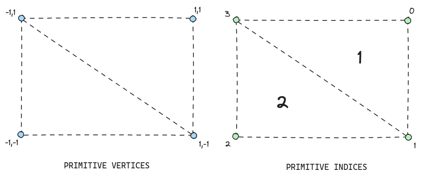
Generating this primitive is relatively trivial, as it only requires setting up the VBO, VAO, and EBO using the following data:
float vertices[] = {
     // positions                       // texture coords
     1.0f,  1.0f, 0.0f,   1.0f, 1.0f,   // top right
     1.0f, -1.0f, 0.0f,   1.0f, 0.0f,   // bottom right
    -1.0f, -1.0f, 0.0f,   0.0f, 0.0f,   // bottom left
    -1.0f,  1.0f, 0.0f,   0.0f, 1.0f    // top left
};

unsigned int indices[] = {
    0, 1, 3, // first triangle
    1, 2, 3  // second triangle
};
In addition to generating and binding the buffers, you must enable the position attribute and the texture coord attribute. Given this, we should now have a pixel buffer which spans the entire fake window.
Pixels as storage #
An issue that becomes apparent regarding the pixel buffer is how exactly will we store floats, when pixels are typically encoded using 1 byte per channel. As it turns out, we do not need to encode floats ourselves, as OpenGL includes a series of floating point textures. Such textures include3:
GL_RGBA32F: each pixel contains 4 32-bit floatsGL_R32F: each pixel contains 1 32-bit floatGL_R16F: each pixel contains 1 16-bit float
We will use GL_RGBA32F, as it allows for a vectorized representation of our data, processing 4 floats per fragment, likely allowing us (best case scenario) to sample our textures once per 4 floats instead of once per each float.
Buffer creation #
Before creating GPU-bound buffers, we need to define a maximum width and height for our window’s pixel buffer, which will act as the largest buffer our library can process. Once again, this is quite a trivial step as it simply requires passing the width and height of our pixel buffer to the GL backend (EGL) to properly configure, the same way we would set the dimensions of a window.
Creating the buffers themselves is as easy as generating a texture and framebuffer and binding the texture to the framebuffer. However, we do not want our textures to always inherit the same dimensions as our pixel buffer, as we will likely process smaller batches of data that don’t share the same dimensions as the pixel buffer, which could be massive and wastes VRAM. As such, we need a function to properly set the dimensions of the textures:
// FLOATS_PER_PIXEL = 4 (RGBA)
static void get_texture_dimensions( size_t size
                                  , int max_width
                                  , int max_height
                                  , int *out_width
                                  , int *out_height
                                  , bool *is_padded )
{
    // transform size to contain number of floats
    size_t count = (size_t)ceilf((float)size / (FLOATS_PER_PIXEL * sizeof(float)));

    if (is_padded)
        *is_padded = roundf((float)size / (FLOATS_PER_PIXEL * sizeof(float)))
                     != ((float)size / (FLOATS_PER_PIXEL * sizeof(float)));

    // check if buffer is tiny
    if (count <= max_width) {
        *out_width = count;
        *out_height = 1;
        return;
    }

    // otherwise, (max_width, variable height)
    *out_width = max_width;
    *out_height = (int)ceilf((float)count / max_width);
}
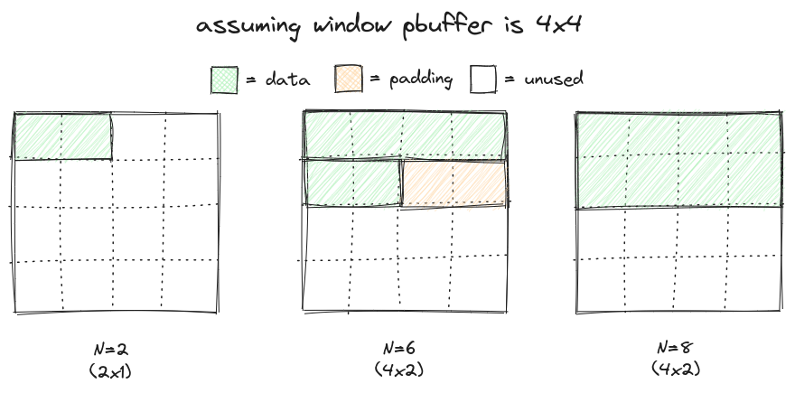
Using this function, we can set the dimensions of our textures according to the size of their respective buffers, saving VRAM.
N refers to the number of floats within our buffer. We add padding so our textures are shaped rectangular. For this image to be completely accurate, multiply the Ns by 4. $$width = \begin{cases} N, & \text{if } N \leq w_{max} \\ w_{max}, & \text{otherwise} \end{cases}$$ $$height = \begin{cases} 1, & \text{if } N \leq w_{max} \\ \lceil \frac{N}{w_{max}} \rceil, & \text{otherwise} \end{cases}$$ $$padded = \begin{cases} 1, & \text{if } \lfloor \frac{\text{size}}{16} \rceil \neq \frac{\text{size}}{16} \\ 0, & \text{otherwise} \end{cases}$$
Copying memory #
To get data to and from our textures, we need to build a specialized memcpy function. Before copying any memory around, we need to prepare the host to either send or receive. This is done by either:
- Host to GPU: Copy
srctosafe_bufferwhose size is based on the max dimensions, thenglTexSubImage2Dinto the texture. - GPU to host: Use
glReadPixelson texture (src) intosafe_buffer, then copy intodstbased on true size, not buffer size.
A safe buffer is required due to potentially reading/writing memory out of bounds. When referring to the previous figure, we can see that both N=6 and N=8 have the same dimensions, however we would copy too much memory into the N=6 buffer if we were attempted to get data back from the GPU. Likewise, we would read out of bounds if we tried copying the N=6 buffer into the texture. By first copying into a safe buffer whose size is the maximum possible, we avoid the risk of memory corruption.
Although a safe buffer avoids the risk of memory corruption, it greatly reduces performance when working with large quantities of data. This is because we would be moving data from the host twice, once to the safe buffer, then to the GPU. We only actually need a safe buffer if there is padding within the texture, since no padding means the buffer the user provides will be the correct size.
Kernels #
With the major components of memory management and headless rendering initialization out of the way, we can begin writing the compute kernels. We base our kernels off of the BLAS specification, which outlines a set of routines for performing linear algebra operations. Note that all the kernels below are prefixed with an s, indicating the use of single precision floats. This conforms with our previously established image format of GL_RGBA32F, which handles 32-bit floats.
saxpy #
Definition #
$$y=\alpha x + y $$
Pseudocode #
saxpy(int N, float alpha, const float *x, int incx, float *y, int incy);
Discussion #
saxpy defines a vector addition operation, in which we add a vector x multiplied by a scalar $\alpha$ to the vector y.
Where the parameters are defined as:
N: Elements inyalpha: Constant to multiply elements inxbyx: Vector xincx: Increment in accesses toxy: Vector yincy: Increment in writes toy
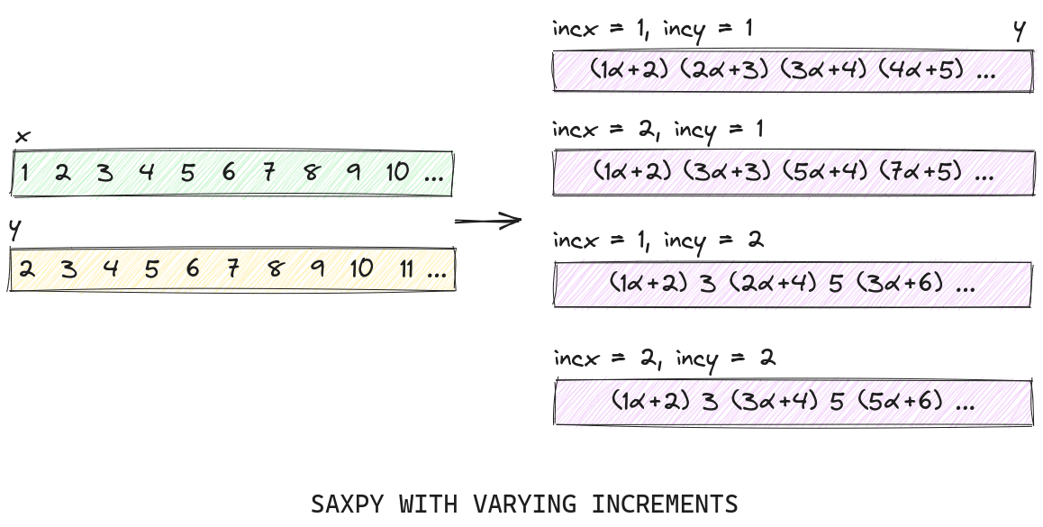
Most of the parameters are self-explanatory as they are a part of the equation provided above. However, two of them stick out: incx and incy. These two variables change how data in the x and y vectors are accessed:
saxpy with varying inc. The inc_ parameters allow for strided data to be accessed accordingly within the same buffer.
Given all this, our fragment shader will have to have access to the following variables:
out vec4 FragColor;    // output vector
in vec2 TexCoord;      // current coordinate/position
uniform sampler2D x;   // x vector
uniform sampler2D y;   // y vector
uniform float alpha;   // alpha
uniform int incx;      // incx
uniform int incy;      // incy
uniform vec2 dims;     // output dimensions (y dims)
uniform int max_index; // N
Because the fragment shader runs once per every fragment, we need to ensure that we understand the position of our fragment relative to the buffer. This is the fragment index, and it can be calculated by:
int index = int(gl_FragCoord.y - 0.5) * int(dims.x) + int(gl_FragCoord.x - 0.5) * 4;
Fragment coordinates are centered at each pixel, meaning subtracting 0.5 from the x and y will give us the pixel coordinate. We multiply by 4 because each fragment contains 4 floats/channels (RGBA). As such, the first fragment will have an index of 0, the second fragment will have an index of 4, etc.
Using this index, we can determine which elements within the current fragment are to be modified, where offs is an integer ranging from [0, 3], indicating the channel to be accessed (R, G, B, A):
if ((index + offs) < max_index && (index + offs) % incy == 0) {
    ...
}
Next, we have to sample the values in the x and y vectors. Sampling the y vector is easy (and done once at the start of the shader), as its texture coordinate is provided by TexCoord:
vec4 vy = texture(y, TexCoord);
Sampling the x vector, though, requires calculating its texture coordinate. If we assumed that incx=1 would always be true, this step could be skipped as you would re-use TexCoord (both vectors would be assumed to be the same dimensions/size). However, this won’t always be the case. As such, we calculate the texture coordinate with respect to the x vector using the current index and the increments:
int xindex = ((index + offs) + ((index + offs) / incy) * (incx - incy));
vec2 coord = vec2(
    float((xindex / 4) % int(dims.x)) / dims.x,
    float((xindex / 4) / int(dims.x)) / dims.y
);
vec4 vx = texture(x, coord);
In the code above, xindex is the index of the individual element, meaning it must be divided by 4 to obtain the fragment index. Performing the modulo using the width (dims.x) gives us the x coordinate, while dividing gives us the y coordinate. We divide the results by the width and height to normalize the coordinate.
As stated before, incx won’t always be 1, meaning we have to extract the specific element from the vector, which is relatively simple. Following this extraction, we can set the output value accordingly, where elem is either r, g, b, or a:
float val;
switch (xindex % 4) {
case 0: val = vx.r; break;
case 1: val = vx.g; break;
case 2: val = vx.b; break;
case 3: val = vx.a; break;
}
vy.elem += val * alpha;
Finally, at the end of our shader, we write the resulting vector to the fragment color:
FragColor = vy;
It should be noted that worst case scenario, we sample our textures 5 times per fragment, possibly degrading performance for operations which don’t have varying increments. As such, texture sampling could be cut down to just 2, if we make a seperate shader whose task is to only handle cases where incx and incy are either both 1 or multiples of 4.
Executing the shader works the same way as executing any other shader, with an extra few steps:
glViewportusing vectory’s internal texture dimensionsglUseProgramonsaxpyglActiveTexture,glBindTexture,glUniform1ionx&yglUniform**to set other variables (incx,alpha, etc…)glBindFramebufferusing vectory’s internal framebufferglBindVertexArrayon previously created globalVAOglDrawElements- If necessary, call
glFinish
With that, the most fundamental operation of vector addition is complete.
sdot #
Definition #
$$result=x \cdot y $$
Pseudocode #
sdot(int N, float *result, const float *x, int incx, const float *y, int incy);
Discussion #
The dot product is an interesting kernel to implement, since the result is a scalar, rather than a vector. A naive implementation may approach this problem with the following implementation, where we calculate the dot product within a single fragment call:
/// pseudocode
void main()
{
    vec4 res = vec4(0, 0, 0, 0);
    if (index == 0) {
        for (int i = 0; i < N / 4; i++) {
          vec4 vx = texture(x, index_to_coord(i));
          vec4 vy = texture(y, index_to_coord(i));
          vec4 vz = vx * vy;
          res.r += vz.r + vz.g + vz.b + vz.a;
        }
    }
    frag = res;
}
This implementation, however, is extremely slow. Instead of making use of the possible thousands of fragments provided, we calculate the result in a single fragment call. Individual fragments aren’t fast enough on their own, which is why they need to be paired with other fragments to make use of parallelism.
As such, we can instead divide the dot product into two distinct operations:
- Multiply vectors
xandy, store into vectorz - Perform summation on vector
z
By splitting the dot product into these two operations, we can maximize parallelism using a single shader call for the first step, and utilizing a technique called reduction for the second step.
Step 1: Multiplication kernel #
There isn’t anything complicated regarding the multiplication kernel. In fact, we can re-use the previously implemented saxpy kernel and change a single line (and remove alpha) to perform multiplication instead of addition.
So, instead of this:
vy.elem += val * alpha;
We have:
vy.elem *= val;
With that, the multiplication portion of the dot product performs with about the same speed as the saxpy kernel.
Step 2: Summation kernel #
The summation operation is where we face our biggest slowdowns. To combat this, our shader employs a technique called reduction, in which per every shader call, we cut the size of our vector in half by adding the second half to the first half repeatedly until we are only left with a single element:
reduction operation. Instead of iterating through each element within a single fragment, we slowly reduce the “size” of the buffer by adding the first half blocks by the second half blocks, and cutting the buffer in half.
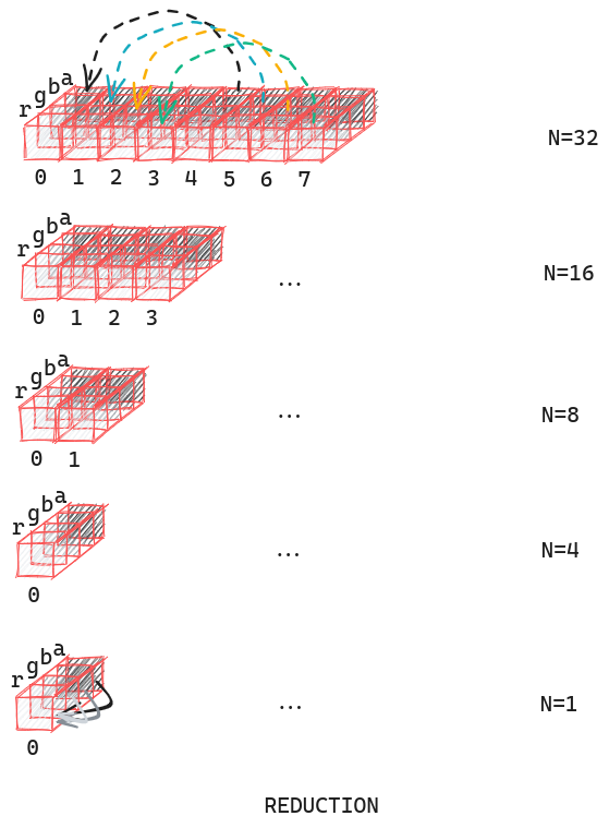
The exact process of reduction within the shader itself is as follows:
- Start with vector
z, sizeN - Divide
Nby two. The shader will go through the first half of fragments, adding the value contained in the fragment whose position isN/2(2)Same value ofN/2as before, notN/4. away from the current fragment. For the fragments in the second half, do nothing. - Repeat step 2 until
N=4 - At
N=4, add up all the values contained in the fragment whose index is0into the red channel.
In pseudocode, the reduction operation looks something like this (without channel vectorization):
for (int i = N; i != 1; i /= 2)
    // kernel
    for (int j = 0; j < i / 2; j++)
        y[j] += y[j+(i/2)];
This means that our reduction summation shader will be called multiple times until we reach the final element.
Improvement #
| N | Vector size | sdot (Sequential) | sdot (Reduction) | Improvement | |
|---|---|---|---|---|---|
| 1024 | 4 KiB | 0.053s | 0.052s | +1.89% | |
| 1048576 | 4 MiB | 0.197s | 0.071s | +63.96% | |
| 67108864 | 256 MiB | 8.338s | 0.477s | +94.28% | |
| 268435456 | 1 GiB | 17.346s | 8.517s | +50.90% |
Although the performance is still quite lackluster with larger vectors, it is a significant improvement from the sequential kernel. It also appears that it may be more effective to split sdot accross multiple calls, like for N=268435456 where its possible to achieve ~1.908s if we split it into four N=67108864 calls, adding the results on the host.
sgemm #
Definition #
$$C=\alpha AB + \beta C $$
Pseudocode #
sgemm( bool aT, bool bT
     , int m, int n, int k, float alpha
     , const float *A, int lda
     , const float *B, int ldb, float beta
     , float *C, int ldc );
Discussion #
The general matrix multiply is challenging function to implement, with regard to achieving the highest performance possible. The implementation of the general matrix multiply kernel could either be:
- Written as a new shader
- Perform
scopy&sdoton every element inC
Of these two options, the former makes the most sense. The latter, although requiring less work, would result in an implementation that is extremely slow with large matrices. This is because we would be making over m*n*4
(3)The 4 comes from the amount of shaders we call: scopy three times, sdot once. m*n is how many elements are in matrix C.
draw calls, as we would copy portions of matrices A and B into vectors, performing the dot product (which has additional draw calls for reduction), and copy the result element by element.
As such, writing a single shader to handle all these operations would be significantly faster, as it would only require a single draw call.
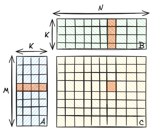
The general matrix multiply operation can be visualized below, where matrices A, B, and C are in column major order:
A and B determine the result of elements in C.
Like previous shaders, we calculate the current index, only sample the C texture if $\beta \neq 0$, and check if the current index plus the current element offset is less than the maximum index. Within the shader, before going into the actual kernels, we first determine the dimensions of our matrices:
int ax = aT ? k : int(adims.x);
int ay = aT ? int(adims.x) : k;
int bx = bT ? int(bdims.y) : k;
int by = bT ? k : int(bdims.y);
These values will come in handy when normalizing our coordinates before sampling. Next, after checking that the current index is less than the maximum, we obtain the current row and column, the same way we convert linear indexes into coordinates:
int i = (index + offs) % m; // row
int j = (index + offs) / m; // col
Next, we perform a dot product on the current element. We do this by looping through K elements, as both matrices A and B share this dimension. We obtain the indexes using the ld* variables, which are effectively strides of the matrices:
float val = 0;
for (int l = 0; l < k; l++) {
    int aindex = aT ? lda * i + l : lda * l + i;
    int bindex = bT ? ldb * l + j : ldb * j + l;
    ...
}
The rest of the kernel logic follows the same principle as the previous kernels; convert the linear indexes into coordinates (divide indexes by 4, coordinate of A normalizes with ax, ay, B w/ bx, by), sample A and B with their respective coordinates, determine which element to access, then multiply the sampled values and add that to val.
In the end, our “dot product” result will be in val, allowing us to finish with the following statement, where vy is either (0, 0, 0, 0) or sampled from C:
vy.elem = (alpha * val) + (vy.elem * beta);
Optimization #
At a glance, it may appear there is little room for optimization, given that I’ve stated earlier that methods like reduction for large matrices don’t work out well with regard to speed due to the extensive draw calls. However, we can employ a different technique for significant speedups, particularly with matrices whose shapes are multiples of 4x4.
The drawback to our current implementation is that we sample matrices A and B about m*n*k times. This is primarily due to how the matrices are ordered vs how they are in memory:
A and B are not transposed.
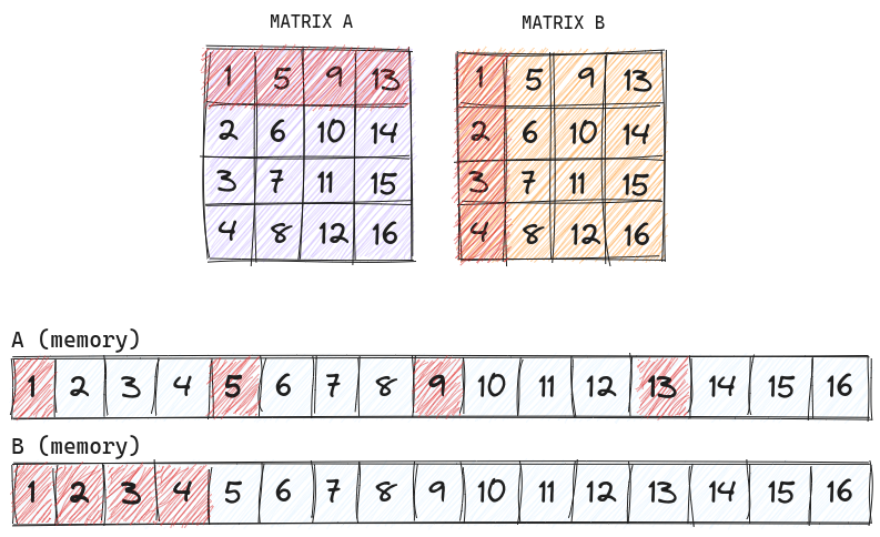
Due to the memory layout of the matrices, A must be sampled 4 times, as opposed to B whose memory layout matches the ordering, allowing us to only sample it once. The solution is to reorder matrix A, such that we can continuously access it the same way we can continuously access matrix B:
A, allowing us to continuously access it in memory, still assuming A and B are not specified to be transposed.
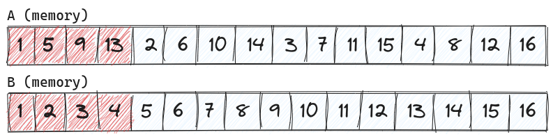
This reordering/transposition allows us to cut down on texture sampling by a factor of 4, meaning our kernel will now only sample A and B about M*N*(K/4) times, significantly cutting down on time spent on the summation.
This reordering is done through another shader, copied into another matrix as to not modify the user’s matrix. Although we now have two draw calls (one to reorder, one performing matrix multiplication) and memory allocation/deallocation, we managed to outperform our original shader. It should be noted that we only need to reorder for these specific cases (dependent on user input regarding transposition):
- Reorder
$A$if$A^T$isfalse - Reorder
$B$if$B^T$istrue
In the end, we see some significant performance gains over the non-optimized shader, particularly with larger matrices.
(4)Attempting to run the V1 kernel on matrices sized 4096x4096 caused graphical issues and would stall out on __sched_yield upon framebuffer/texture deletion, requiring user intervention to close the program.
However, like the sdot shader, we still see somewhat lackluster performance with larger data, indicating there are likely more optimizations to be made.
| Dimensions | Matrix size | sgemm (1x1) | sgemm (4x4) | Improvement | |
|---|---|---|---|---|---|
| 64x64 | 16 KiB | 0.053s | 0.050s | +5.66% | |
| 512x512 | 1 MiB | 0.087s | 0.067s | +22.99% | |
| 1024x1024 | 4 MiB | 0.261s | 0.115s | +55.94% | |
| 2048x2048 | 16 MiB | 1.589s | 0.375s | +76.40% | |
| 4096x4096 | 64 MiB | ~12s * | 2.437s | +79.69% |
Results #
The results
(5)Tests were performed on Linux (using DE) using a GeForce GTX 1050 (545.29.06, CUDA Version: 12.3)
below are a measure of each of the respective program’s entire runtime. This is done to not only benchmark the kernels themselves, but the speed of memory transfer (cudaMemcpy vs glblasMemcpy) aswell.
| Demo | N | Vector/Matrix size | cuBLAS | glBLAS | Improvement |
|---|---|---|---|---|---|
| saxpy | 1024 | 4 KiB | 0.138s | 0.083s | +39.86% |
| saxpy | 1048576 | 4 MiB | 0.150s | 0.100s | +33.33% |
| saxpy | 67108864 | 256 MiB | 0.483s | 0.371s | +23.19% |
| saxpy | 268435456 | 1 GiB | 1.877s | 1.313s | +30.05% |
| sdot | 1024 | 4 KiB | 0.151s | 0.052s | +65.56% |
| sdot | 1048576 | 4 MiB | 0.152s | 0.071s | +53.27% |
| sdot | 67108864 | 256 MiB | 0.403s | 0.477s | -18.36% |
| sdot | 268435456 | 1 GiB | 1.556s | 8.517s | -447.37% |
| sgemm | 64x64 | 16 KiB | 0.135s | 0.050s | +62.96% |
| sgemm | 512x512 | 1 MiB | 0.134s | 0.067s | +50.00% |
| sgemm | 1024x1024 | 4 MiB | 0.136s | 0.115s | +15.44% |
| sgemm | 4096x4096 | 64 MiB | 0.335s | 2.377s | -609.55% |
Observations #
During the benchmarking process, an interesting issue arose regarding the implementation of glblasMemcpy, particularly focusing on uploading buffers from the host to the GPU. The function call to glTexSubImage2D is typically fast enough that for large buffers (e.g) 8192x8192x4 that the delay is quite small, averaging about 0.34 seconds, but in some scenarios (possibly extended uptimes, rerunning the program too many times, driver issues, not freeing textures/framebuffers, etc.) this delay can jump up to 1.5 seconds, leading to undesirable benchmark results. Moving data from the GPU back to the host seemed unaffected, as it calls glReadPixels.
Another issue that arose was my entire system briefly lagging when running the sdot demo with N=268435456. This behavior isn’t mysterious, as an anticipated side effect to running compute over the rendering pipeline is taking away resources from rendering everything else on the screen, despite running headlessly.
The same issue was experienced with running the sgemm demo using the non-4x4 implementation, in which the system would briefly lag and even (rarely) crash another graphical application. Unlike the sdot demo, however, it would not close on its own. When debugging, I had found that it stalled at __sched_yield, with the call stack indicating the call was to glDeleteFramebuffers.
Closing remarks #
Reflecting on all that has been discussed, running compute intensive calculations through the rendering pipeline is clearly possible. Writing performant and functional kernels purely in fragment shaders, however, is quite a pain. Drivers across different vendors have their own respective quirks, meaning unless extensively tested, this project could have very inconsitent performance. Even on the same system, the benchmarks can become skewed as it appears the demos begin to slow down with extended uptimes. These inconsistencies are coupled with the fact that these kernels hog the graphics pipeline when processing large amounts of data for extended periods of time, taking away resources from other graphical tasks.
Nonetheless compute over fragment shaders proved to be quite viable for small to medium-sized data. As for the larger batches of data, you would want to stick to real compute libraries.